DenseNet vs Fashion MNIST

Implement the DenseNet to showcase is superiority over the ResNet

Dense-Net Architecture

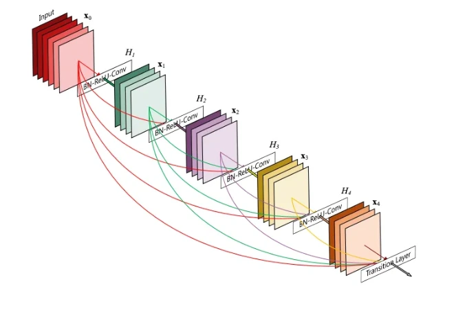
For deep neural networks, as the input get convoluted and processed by many prior layers the deeper layers begin to loose the original input data and receive more noise as a result, training times take significantly longer and the CNN can perform worse. ResNets solve this issue by using skip connections meaning deeper layers receive less noise, however DenseNets solve this issue by essentially using more connections than ResNets. For each dense Block in the network, they take the output of prior dense blocks results as input. This means that even the deepest dense block is receiving input data with very little noise in comparison.

The core idea behind the DenseNet architecture is that the feature maps produced by each layer can be concatenated to form the input to the next layer. This means that the output of each layer is the input of all the following layers. DenseNet also uses a transition layer between each dense block to reduce the spatial dimensionality and the number of feature maps. The transition layer consists of a batch normalisation layer, a 1x1 convolutional layer, and a pooling layer.

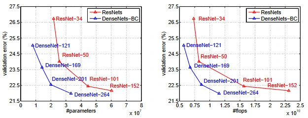
As a result compared with the comparable ResNets the Dense Nets seem to require less to training to achieve higher accuracy results in the ImageNet Validation.

Explanation of Code

Packages

This implementation of the dense net is done using PyTorch. The PyTorch Data Loader is used for data Augmentation.

import torch
import torch.nn as nn
import torch.optim as optim
import torchvision
import torchvision.transforms as transforms
from torchvision.datasets import FashionMNIST
from torch.utils.data import DataLoader
from torchvision import datasets, transforms
import matplotlib.pyplot as plt

Data Processing and Augmentation

For train_dataset there was option to augment the data as seen in the # transformations = transforms.Compose([]) function, however any attempt to augment the Fashion MNIST training data with normalisation resulted in a large and significant decrease in accuracy even after a very large number of epochs. Attempting augmentation without normalisation did produce good results:

Train Loss: 0.2944
Test Loss: 0.3079
Train Accuracy: 89.14%
Test Accuracy: 89.90%

However they are inferior to the results I obtained without augmenting the data. For this reason I have decided against augmenting the data

num_epochs = 50
num_classes = 10
batch_size = 64
learning_rate = 0.001

# Device configuration
device = torch.device('cuda' if torch.cuda.is_available() else 'cpu')
 
num_epochs = 50
num_classes = 10
batch_size = 64
learning_rate = 0.001
 
# AUGMENTATION # redacted
 
# transformations = transforms.Compose([
#     transforms.RandomHorizontalFlip(),
#     transforms.RandomVerticalFlip(),
#     transforms.RandomRotation(10),
#     transforms.RandomResizedCrop(28, scale=(0.8, 1.0)),
#     transforms.RandomPerspective(distortion_scale=0.2, p=0.2),
#     transforms.RandomAffine(degrees=0, translate=(0.1, 0.1), scale=(0.8, 1.2), shear=10),
#     transforms.GaussianBlur(kernel_size=(3, 3), sigma=(0.1, 2.0)),
#     transforms.Normalize((0.5,), (0.5,)),
#     transforms.RandomErasing(),
#     transforms.Pad(padding=2),
#     transforms.CenterCrop(28),
#     transforms.ToTensor(),
# ])
 
# # Create the train dataset with the transformations
# train_dataset = datasets.FashionMNIST(root='./data', 
#                                       train=True, 
#                                       transform=transformations, 
#                                       download=True)
 
# Fashion MNIST dataset
 
#data augmentation
train_dataset = FashionMNIST(root='./data',
                              train=True,
                              transform=transforms.ToTensor(),
                              download=True)
 
test_dataset = FashionMNIST(root='./data',
                            train=False,
                            transform=transforms.ToTensor())
 
# Data loader
train_loader = DataLoader(dataset=train_dataset,
                          batch_size=batch_size,
                          shuffle=True)
 
test_loader = DataLoader(dataset=test_dataset,
                         batch_size=batch_size,
                         shuffle=False)

DenseNet Block

Batch Normalization self.bn: This layer normalizes the inputs for each mini-batch. It helps in stabilising the learning process and speeds up the convergence of the training. (This is different from the normalising mentioned above for augmentation purposes).
ReLU Activation self.relu: a non-linear activation function. It introduces non-linearity into the model, allowing it to learn more complex patterns. The inplace = True argument optimizes memory usage.
Convolutional Layer self.conv: This layer performs a convolution operation. It is a fundamental part of CNNs (Convolutional Neural Networks) and is used to extract features from the input data. The convolution here uses a kernel size of 3x3, padding of 1 (to maintain the spatial dimensions), and no bias term. A lot of the inspiration for the dense net came from this [4].

# DenseNet Block
class DenseBlock(nn.Module):
    def __init__(self, in_channels, growth_rate):
        super(DenseBlock, self).__init__()
        self.bn = nn.BatchNorm2d(in_channels)
        self.relu = nn.ReLU(inplace=True)
        self.conv = nn.Conv2d(in_channels, growth_rate, kernel_size=3, padding=1, bias=False)
        
    def forward(self, x):
        out = self.conv(self.relu(self.bn(x)))
        out = torch.cat([x, out], 1)
        return out

Transition Layer

The TransitionLayergets some data (x), it first smoothens it out (batch normalization), makes some key decisions (ReLU), picks out the important features (convolution), and then compresses this

# Transition Layer
class TransitionLayer(nn.Module):
    def __init__(self, in_channels, out_channels):
        super(TransitionLayer, self).__init__()
        self.bn = nn.BatchNorm2d(in_channels)
        self.relu = nn.ReLU(inplace=True)
        self.conv = nn.Conv2d(in_channels, out_channels, kernel_size=1, bias=False)
        self.avg_pool = nn.AvgPool2d(kernel_size=2, stride=2)
 
    def forward(self, x):
        out = self.conv(self.relu(self.bn(x)))
        out = self.avg_pool(out)
        return out

In DenseNet, these TransitionLayer blocks act as bridges between different dense blocks. They help in controlling the size of the feature maps, ensuring that the network doesn’t get too heavy and slow to process as it gets deeper. It's like having a checkpoint or a rest area in a long highway, keeping things in order and manageable.

Dense Blocks and Transition layers:

The DenseBlock and TransitionLayer are the core components. The dense blocks focus on extracting a rich set of features, building upon what was learned in the previous layers. It's like each block adds a layer of understanding, picking up more and more details.
The transition layers, on the other hand, help in streamlining this information, making sure it's not too overwhelming as it moves deeper into the network.

Final Processing and Classification:

After going through the dense and transition layers, the data undergoes final processing (self.relu([self.bn](http://self.bn/)(out))), ensuring it's in the best form for the final decision-making.
The self.avg_pool then compresses the data to a size that's easier to work with, focusing on the essence of what's been learned.
Finally, self.fc is a fully connected layer that takes all this processed information and translates it into specific class predictions.

# DenseNet Model
class DenseNet(nn.Module):
    def __init__(self, num_classes):
        super(DenseNet, self).__init__()
 
        self.init_conv = nn.Conv2d(1, 16, kernel_size=7, stride=2, padding=3, bias=False)
 
        # Dense Blocks and Transition Layers
        self.dense1 = DenseBlock(16, 16)
        self.trans1 = TransitionLayer(32, 32)
        self.dense2 = DenseBlock(32, 32)
        self.trans2 = TransitionLayer(64, 64)
 
        self.bn = nn.BatchNorm2d(64)
        self.relu = nn.ReLU(inplace=True)
        self.avg_pool = nn.AdaptiveAvgPool2d((1, 1))
        self.fc = nn.Linear(64, num_classes)
 
    def forward(self, x):
        out = self.init_conv(x)
        out = self.trans1(self.dense1(out))
        out = self.trans2(self.dense2(out))
        out = self.relu(self.bn(out))
        out = self.avg_pool(out)
        out = out.view(out.size(0), -1)
        out = self.fc(out)
        return out
 
model = DenseNet(num_classes=num_classes).to(device)

Training and Optimising the model

Cross-Entropy Loss: This is your criterion for measuring how well the model is performing. It's like a teacher grading an exam, showing where the model needs to improve.
Adam Optimizer: This is like the coach for your model, guiding the learning process by adjusting weights to reduce errors (loss).

# Loss and optimizer
criterion = nn.CrossEntropyLoss()
optimizer = optim.Adam(model.parameters(), lr=learning_rate)

Explanation of Implementation

model.train() sets the model to training mode, enabling features like dropout and batch normalization specific to this phase.

running_loss, correct, and total are initialized to track the loss and accuracy during the epoch. The inner loop iterates over the training data loader train_loader , fetching batches of images and their corresponding labels.

[images.to](http://images.to/)(device) and [labels.to](http://labels.to/)(device) ensure that the data is moved to the GPU if available. The forward pass computes the model's predictions outputs and calculates the loss using criterion.

The backward pass loss.backward() computes the gradient of the loss, and optimizer.step() updates the model's weights. Running loss and accuracy statistics are updated after each batch. This is then repeated x number of epochs that is pre defined.

for epoch in range(num_epochs):
    model.train()
    running_loss = 0.0
    correct = 0
    total = 0
    for i, (images, labels) in enumerate(train_loader):
        images = images.to(device)
        labels = labels.to(device)
        
        # Forward pass
        outputs = model(images)
        loss = criterion(outputs, labels)
 
        # Backward and optimize
        optimizer.zero_grad()
        loss.backward()
        optimizer.step()
 
        running_loss += loss.item()
        _, predicted = torch.max(outputs.data, 1)
        total += labels.size(0)
        correct += (predicted == labels).sum().item()
 
        if (i+1) % 100 == 0:
            print(f'Epoch [{epoch+1}/{num_epochs}], Step [{i+1}/{total_step}], Loss: {loss.item():.4f}')
 
    train_losses.append(running_loss / total_step)
    train_accuracies.append(100 * correct / total)
 
    # Test the model
    model.eval()
    running_loss = 0.0
    correct = 0
    total = 0
    with torch.no_grad():
        for images, labels in test_loader:
            images = images.to(device)
            labels = labels.to(device)
            outputs = model(images)
            loss = criterion(outputs, labels)
            running_loss += loss.item()
            _, predicted = torch.max(outputs.data, 1)
            total += labels.size(0)
            correct += (predicted == labels).sum().item()
 
    test_losses.append(running_loss / len(test_loader))
    test_accuracies.append(100 * correct / total)
    
        print(f'Epoch [{epoch+1}/{num_epochs}], Train Loss: {train_losses[-1]:.4f}, Test Loss: {test_losses[-1]:.4f}, Train Accuracy: {train_accuracies[-1]:.2f}%, Test Accuracy: {test_accuracies[-1]:.2f}%')
 
# Save the model checkpoint
torch.save(model.state_dict(), 'model.ckpt')

Results

# Plotting training and testing losses
plt.figure(figsize=(12, 4))
plt.subplot(1, 2, 1)
plt.plot(train_losses, label='Train Loss')
plt.plot(test_losses, label='Test Loss')
plt.title('Loss per Epoch')
plt.xlabel('Epoch')
plt.ylabel('Loss')
plt.legend()
 
# Plotting training and testing accuracies
plt.subplot(1, 2, 2)
plt.plot(train_accuracies, label='Train Accuracy')
plt.plot(test_accuracies, label='Test Accuracy')
plt.title('Accuracy per Epoch')
plt.xlabel('Epoch')
plt.ylabel('Accuracy')
plt.legend()
plt.show()
 
print(train_losses)
print(test_losses)
print(test_accuracies)
print(train_accuracies)

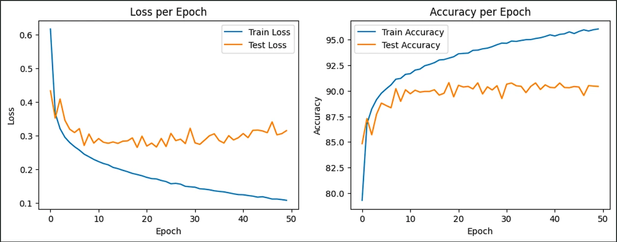
At 50 Epochs:

Train Loss: 0.1115
Test Loss: 0.3022
Train Accuracy: 95.84%
Test Accuracy: 90.51%

Conclusion

Overall I am happy with the result and implementation of the dense net, comparing my results from standard benchmarks like the ResNet18 (Accuracy = 94.9%) and DenseNet-BC 768K params (accuracy = 95.4% ) . Given I used significantly less params with a significant decrease in training time and hardware, a test accuracy of 90.51% is a success.[5]

From the results you can see that ~10 epochs not much changed in terms of test-accuracy and test loss. When running test after 50 epochs although the training accuracy still continued to increase, the test accuracy and loss began to diminish, this is probably due to overtraining and so, 50 epochs seems to be an accurate number of iterations to train the DenseNet. Looking closely at the test loss you can see a small increment in the general trends from ~20 epoch, indicating the test accuracy of 90.51% is around the best the network can do. Looking closely at the accuracy graph after ~10 epochs no general change in the the test accuracy can be noticed

To increase test accuracy, augmentation of the data in a specific way, may of helped however as mentioned earlier, augmenting the data seemed to decrease accuracy. Another way of increasing accuracy potentially, is to increase the number of params the model takes, more data will make the network perform better.

References

[1] Medium, "Understanding and coding a ResNet in Keras," [Online]. Available:https://miro.medium.com/v2/resize:fit:1100/format:webp/1*jm5MEylOA8abyAi51CcSLA.png. [Accessed: Dec. 1, 2023].

[2] Towards Data Science, "Image Classification, Transfer Learning, and Fine Tuning using TensorFlow," [Online]. Available:https://towardsdatascience.com/image-classification-transfer-learning-and-fine-tuning-using-tensorflow-a791baf9dbf3. [Accessed: Dec. 3, 2023].

[3] A. Kolesnikov, L. Beyer, X. Zhai, J. Puigcerver, J. Yung, S. Gelly, and N.Houlsby, "Big Transfer (BiT): General Visual Representation Learning," arXiv:1905.11946, 2019. [Online]. Available: https://arxiv.org/pdf/1905.11946.pdf.

[4] K. He, X. Zhang, S. Ren, and J. Sun, "Deep Residual Learning for Image Recognition," arXiv:1608.06993, 2016. [Online]. Available: https://arxiv.org/pdf/1608.06993.pdf.

[5] Papers With Code, "SOTA for Image Classification on Fashion-MNIST," [Online].Available: https://paperswithcode.com/sota/image-classification-on-fashion-mnist.[Accessed: Dec. 1, 2023].